qPicture descriptions:
qRaster:
qCompletely
specified by the
set of intensities for the pixels positions in the display.
qShapes and colors are described
with pixel
arrays.
qScene displayed by loading pixels
array into the frame buffer.
qVector:
qSet of complex objects
positioned at specified coordinates locations within
the scene.
qShapes and colors are described
with sets
of basic geometric structures.
qScene is displayed by scan
converting the
geometric-structure specifications into pixel patterns.
qOutput Primitives:
q Basic geometric structures used to
describe scenes.
q Can be grouped into
more complex
structures.
q Each one is specified with input
coordinate data
and other information about the way that object is to be displayed.
q Examples: point, line and
circle each one with specified coordinates.
q Construct the vector picture.
In digital
representation:
qDisplay screen is divided into scan
lines and columns.
qPixels positions are referenced according to scan line number and column number (columns across scan
lines).
qScan lines start from 0 at screen bottom, and columns start from 0 at the screen left side.
qScreen locations (or pixels)
are referenced with integer
values.
qThe frame buffer stores the intensities temporarily.
qVideo controller reads from the frame buffer and plots the screen pixels.
- Attributes of Output Primitives
Any parameter that affects the way a primitive is to be displayed is referred to as an attribute parameter. Example attribute parameters are color, size etc. A line drawing function for example could contain parameter to set color, width and other properties.
1. Line Attributes
2. Curve Attributes
3. Color and Grayscale Levels
4. Area Fill Attributes
5. Character Attributes
6. Bundled Attributes
Line Attributes
Basic attributes of a straight line segment are its type, its width, and its color. In some graphics packages, lines can also be displayed using selected pen or brush options
* Line Type
* Line Width
* Pen and Brush Options
* Line Color
Line type
Possible selection of line type attribute includes solid lines, dashed lines and dotted lines. To set line type attributes in a PHIGS application program, a user invokes the function
setLinetype (lt)
Where parameter lt is assigned a positive integer value of 1, 2, 3 or 4 to generate lines that are solid, dashed, dash dotted respectively. Other values for line type parameter it could be used to display variations in dot-dash patterns.
Line width
Implementation of line width option depends on the capabilities of the output device to set the line width attributes.
setLinewidthScaleFactor (lw)
Line width parameter lw is assigned a positive number to indicate the relative width of line to be displayed. A value of 1 specifies a standard width line. A user could set lw to a value of 0.5 to plot a line whose width is half that of the standard line. Values greater than 1 produce lines thicker than the standard.
Line Cap
We can adjust the shape of the line ends to give them a better appearance by adding line caps.
There are three types of line cap. They are
* Butt cap
* Round cap
* Projecting square cap
Butt cap obtained by adjusting the end positions of the component parallel lines so that the thick line is displayed with square ends that are perpendicular to the line path.
Round cap obtained by adding a filled semicircle to each butt cap. The circular arcs are centered on the line endpoints and have a diameter equal to the line thickness.
Projecting square cap extend the line and add butt caps that are positioned one-half of the line width beyond the specified endpoints.

Three possible methods for smoothly joining two line segments
* Mitter Join
* Round Join
* Bevel Join
A miter join accomplished by extending the outer boundaries of each of the two lines
until they meet.
A round join is produced by capping the connection between the two segments with a circular boundary whose diameter is equal to the width.
A bevel join is generated by displaying the line segment with but caps and filling in tri
angular gap where the segments meet.

Pen and Brush Options
With some packages, lines can be displayed with pen or brush selections. Options in this category include shape, size, and pattern. Some possible pen or brush shapes are given in Figure
With some packages, lines can be displayed with pen or brush selections. Options in this category include shape, size, and pattern. Some possible pen or brush shapes are given in Figure

Line color
A poly line routine displays a line in the current color by setting this color value in the frame buffer at pixel locations along the line path using the set pixel procedure.
We set the line color value in PHlGS with the function
setPolylineColourIndex (lc)
Nonnegative integer values, corresponding to allowed color choices, are assigned to the line color parameter lc
Example: Various line attribute commands in an applications program is given by the following sequence of statements
setLinetype(2);
setLinewidthScaleFactor(2);
setPolylineColourIndex (5);
polyline(n1, wc points1);
setPolylineColorIindex(6);
poly line (n2, wc points2);
This program segment would display two figures, drawn with double-wide dashed lines. The first is displayed in a color corresponding to code 5, and the second in color 6.
Curve attributes
Parameters for curve attribute are same as those for line segments. Curves displayed with varying colors, widths, dot – dash patterns and available pen or brush options
Color and Grayscale Levels
Various color and intensity-level options can be made available to a user, depending on the capabilities and design objectives of a particular system
In a color raster system, the number of color choices available depends on the amount of storage provided per pixel in the frame buffer
Color-information can be stored in the frame buffer in two ways:
* We can store color codes directly in the frame buffer
* We can put the color codes in a separate table and use pixel values as an index into this table
With the direct storage scheme, whenever a particular color code is specified in an application program, the corresponding binary value is placed in the frame buffer for each-component pixel in the output primitives to be displayed in that color.
A minimum number of colors can be provided in this scheme with 3 bits of storage per pixel, as shown in Table
3 bits - 8 choice of color
6 bits – 64 choice of color
8 bits – 256 choice of color
A user can set color-table entries in a PHIGS applications program with the function
setColourRepresentation (ws, ci, colorptr)
Parameter ws identifies the workstation output device; parameter ci specifies the color index, which is the color-table position number (0 to 255) and parameter colorptr points to a trio of RGB color values (r, g, b) each specified in the range from 0 to 1
Grayscale
With monitors that have no color capability, color functions can be used in an application program to set the shades of gray, or grayscale, for displayed primitives. Numeric values over the range from 0 to 1 can be used to specify grayscale levels, which are then converted to appropriate binary codes for storage in the raster.

Intensity = 0.5[min(r, g, b) + max(r, g, b)]
Area fill Attributes
Options for filling a defined region include a choice between a solid color or a pattern fill and choices for particular colors and patterns
Fill Styles
Areas are displayed with three basic fill styles: hollow with a color border, filled with a solid color, or filled with a specified pattern or design. A basic fill style is selected in a PHIGS program with the function
setInteriorStyle (fs)
Values for the fill-style parameter fs include hollow, solid, and pattern. Another value for fill style is hatch, which is used to fill an area with selected hatching patterns-parallel lines or crossed lines

The color for a solid interior or for a hollow area
outline is chosen with where fill color parameter fc is set to the desired
color code
setInteriorColourIndex (fc)
Pattern Fill
We select fill patterns with setInteriorStyleIndex (pi) where pattern index parameter pi specifies a table position
For example, the following set of statements would fill the area defined in the fillArea command with the second pattern type stored in the pattern table:
SetInteriorStyle( pattern)
SetInteriorStyleIndex(2);
Fill area (n, points)

Character Attributes
The appearance of displayed character is controlled by attributes such as font, size, color and orientation. Attributes can be set both for entire character strings (text) and for individual characters defined as marker symbols
Text Attributes
The choice of font or type face is set of characters with a particular design style as courier, Helvetica, times roman, and various symbol groups.
The characters in a selected font also be displayed with styles. (solid, dotted, double) in bold face in italics, and in outline or shadow styles.
A particular font and associated stvle is selected in a PHIGS program by setting an
integer code for the text font parameter tf in the function
setTextFont (tf)
Control of text color (or intensity) is managed from an application program with
setTextColourIndex (tc)
Where text color parameter tc specifies an allowable color code.
Text size can be adjusted without changing the width to height ratio of characters with
setCharacterHeight (ch)

Parameter ch is assigned a real value greater than 0 to
set the coordinate height of capital letters
The width only of text can be set with function.
setCharacterExpansionFactor (cw)
Where the character width parameter cw is set to a positive real value that scales the body width of character
The width only of text can be set with function.
setCharacterExpansionFactor (cw)
Where the character width parameter cw is set to a positive real value that scales the body width of character

Spacing between characters is controlled separately with
setCharacterSpacing (cs)
Where the character-spacing parameter cs can he assigned any real value
setCharacterSpacing (cs)
Where the character-spacing parameter cs can he assigned any real value

The orientation for a displayed character string is set
according to the direction of the character up vector
setCharacterUpVector (upvect)
Parameter upvect in this function is assigned two values that specify the x and y vector components. For example, with upvect = (1, 1), the direction of the up vector is 45o and text would be displayed as shown in Figure.
setCharacterUpVector (upvect)
Parameter upvect in this function is assigned two values that specify the x and y vector components. For example, with upvect = (1, 1), the direction of the up vector is 45o and text would be displayed as shown in Figure.

To arrange character strings vertically or horizontally
setTextPath (tp)
can be assigned the value: right, left, up, or down
setTextPath (tp)
can be assigned the value: right, left, up, or down


Another handy attribute for character strings is
alignment. This attribute specifies how text is to be positioned with respect
to the $tart coordinates. Alignment attributes are set with
setTextAlignment (h,v)
where parameters h and v control horizontal and vertical alignment. Horizontal alignment is set by assigning h a value of left, center, or right. Vertical alignment is set by assigning v a value of top, cap, half, base or bottom.
A precision specification for text display is given with
setTextPrecision (tpr)
tpr is assigned one of values string, char or stroke.
Marker Attributes
A marker symbol is a single character that can he displayed in different colors and in different sizes. Marker attributes are implemented by procedures that load the chosen character into the raster at the defined positions with the specified color and size. We select a particular character to be the marker symbol with
setMarkerType (mt)
where marker type parameter mt is set to an integer code. Typical codes for marker type are the integers 1 through 5, specifying, respectively, a dot (.) a vertical cross (+), an asterisk (*), a circle (o), and a diagonal cross (X).
We set the marker size with
setMarkerSizeScaleFactor (ms)
with parameter marker size ms assigned a positive number. This scaling parameter is applied to the nominal size for the particular marker symbol chosen. Values greater than 1 produce character enlargement; values less than 1 reduce the marker size.
Marker color is specified with
setPolymarkerColourIndex (mc)
A selected color code parameter mc is stored in the current attribute list and used to display subsequently specified marker primitives
Bundled Attributes
The procedures considered so far each function reference a single attribute that specifies exactly how a primitive is to be displayed these specifications are called individual attributes.
A particular set of attributes values for a primitive on each output device is chosen by specifying appropriate table index. Attributes specified in this manner are called bundled attributes. The choice between a bundled or an unbundled specification is made by setting a switch called the aspect source flag for each of these attributes
setIndividualASF( attributeptr, flagptr)
where parameter attributer ptr points to a list of attributes and parameter flagptr points to the corresponding list of aspect source flags. Each aspect source flag can be assigned a value of individual or bundled.
Bundled line Attributes
Entries in the bundle table for line attributes on a specified workstation are set with the function
setPolylineRepresentation (ws, li, lt, lw, lc)
Parameter ws is the workstation identifier and line index parameter li defines the bundle table position. Parameter lt, lw, tc are then bundled and assigned values to set the line type, line width, and line color specifications for designated table index.
Example
setPolylineRepresentation (1, 3, 2, 0.5, 1)
setPolylineRepresentation (4, 3, 1, 1, 7)
A poly line that is assigned a table index value of 3 would be displayed using dashed lines at half thickness in a blue color on work station 1; while on workstation 4, this same index generates solid, standard-sized white lines
Bundle area fill Attributes
Table entries for bundled area-fill attributes are set with
setInteriorRepresentation (ws, fi, fs, pi, fc)
Which defines the attributes list corresponding to fill index fi on workstation ws. Parameter fs, pi and fc are assigned values for the fill style pattern index and fill color.
Bundled Text Attributes
setTextRepresentation (ws, ti, tf, tp, te, ts, tc)
Bundles values for text font, precision expansion factor size an color in a table position for work station ws that is specified by value assigned to text index parameter ti.
Bundled marker Attributes
setPolymarkerRepresentation (ws, mi, mt, ms, mc)
That defines marker type marker scale factor marker color for index mi on workstation ws.
Inquiry functions
Current settings for attributes and other parameters as workstations types and status in the system lists can be retrieved with inquiry functions.
inquirePolylineIndex ( lastli)
and
inquireInteriorcColourIndex (lastfc)
Copy the current values for line index and fill color into parameter lastli and lastfc.
Two Dimensional Geometric Transformations
Changes in orientations, size and shape are accomplished with geometric transformations that alter the coordinate description of objects.
Basic transformation
* Translation
> T(tx, ty)
> Translation distances
* Scale
> S(sx,sy)
> Scale factors
* Rotation
> R( )
> Rotation angle
Translation
A translation is applied to an object by representing it along a straight line path from one coordinate location to another adding translation distances, tx, ty to original coordinate position (x,y) to move the point to a new position (x’,y’) to
x’ = x + tx, y’ = y + ty
The translation distance point (tx,ty) is called translation vector or shift vector.
Translation equation can be expressed as single matrix equation by using column vectors to represent the coordinate position and the translation vector as


Moving a polygon from one position to another position
with the translation vector (-5.5, 3.75)
Rotations:
A two-dimensional rotation is applied to an object by repositioning it along a circular path on xy plane. To generate a rotation, specify a rotation angle θ and the position (xr, yr) of the rotation point (pivot point) about which the object is to be rotated.
Positive values for the rotation angle define counter clock wise rotation about pivot point. Negative value of angle rotate objects in clock wise direction. The transformation can also be described as a rotation about a rotation axis perpendicular to xy plane and passes through pivot point

Rotation of a point from position (x, y) to position (x’,
y’) through angle θ relative to coordinate origin
The transformation equations for rotation of a point position P when the pivot point is at coordinate origin. In figure r is constant distance of the point positions Ф is the original angular of the point from horizontal and θ is the rotation angle.
The transformed coordinates in terms of angle θ and Ф
x’ = rcos(θ+Ф) = rcosθ cosФ – rsinθsinФ
y’ = rsin(θ+Ф) = rsinθ cosФ + rcosθsinФ
The original coordinates of the point in polar coordinates
x = rcosФ, y = rsinФ
the transformation equation for rotating a point at position (x,y) through an angle θ about origin
x’ = xcosθ – ysinθ
y’ = xsinθ + ycosθ
Rotation Equation
P’ = R . P
Rotation Matrix

Note: Positive values
for the rotation angle define counterclockwise rotations about the rotation
point and negative values rotate objects in the clockwise.
Scaling
A scaling transformation alters the size of an object. This operation can be carried out for polygons by multiplying the coordinate values (x, y) to each vertex by scaling factor Sx & Sy to produce the transformed coordinates (x’, y’)
x’ = x.Sx y’ = y.Sy
scaling factor Sx scales object in x direction while Sy scales in y direction.
The transformation equation in matrix form

(or)
P’ = S. P
Where S is 2 by 2 scaling matrix
P’ = S. P
Where S is 2 by 2 scaling matrix

Turning a square (a) Into a rectangle (b) with scaling factors sx = 2 and
sy = 1.
Any positive numeric values are valid for scaling factors sx and sy. Values less than 1 reduce the size of the objects and values greater than 1 produce an enlarged object.
There are two types of Scaling. They are
* Uniform scaling
* Non Uniform Scaling
To get uniform scaling it is necessary to assign same value for sx and sy. Unequal values for sx and sy result in a non uniform scaling.
Matrix Representation and Homogeneous Coordinates
Many graphics applications involve sequences of geometric transformations. An animation, for example, might require an object to be translated and rotated at each increment of the motion. In order to combine sequence of transformations we have to eliminate the matrix addition. To achieve this we have represent matrix as 3 X 3 instead of 2 X 2 introducing an additional dummy coordinate h. Here points are specified by three numbers instead of two. This coordinate system is called as Homogeneous coordinate system and it allows to express transformation equation as matrix multiplication
Cartesian coordinate position (x, y) is represented as homogeneous coordinate triple (x, y, h)
* Represent coordinates as (x, y, h)
* Actual coordinates drawn will be (x/h, y/h)
For Translation

For Scaling

For Rotation

Composite Transformations
A composite transformation is a sequence of transformations; one followed by the other. we can set up a matrix for any sequence of transformations as a composite transformation matrix by calculating the matrix product of the individual transformations
Translation
If two successive translation vectors (tx1,ty1) and (tx2,ty2) are applied to a coordinate position P, the final transformed location P’ is calculated as
P’ = T(tx2, ty2). {T(tx1, ty1).P}
= {T(tx2, ty2).T(tx1,ty1)}.P
Where P and P’ are represented as homogeneous-coordinate column vectors.
(or)
T(tx2, ty2).T(tx1,ty1) = T(tx1+tx2, ty1+ty2)
Which demonstrated the two successive translations are additive.
Rotations
Two successive rotations applied to point P produce the transformed position
P’ = R(θ2).{R(θ1).P} = {R(θ2).R(θ1)}.P
By multiplying the two rotation matrices, we can verify that two successive rotation are additive
R(θ2).R(θ1) = R(θ1 + θ2)
So that the final rotated coordinates can be calculated with the composite rotation matrix as
P’ = R(θ1 + θ2).P

Scaling
Concatenating transformation matrices for two successive scaling operations produces the following composite scaling matrix
Concatenating transformation matrices for two successive scaling operations produces the following composite scaling matrix

General Pivot-Point Rotation
1. Translate the object so that pivot-position is moved to the coordinate origin
2. Rotate the object about the coordinate origin
Translate the object so that the pivot point is returned to its original position
1. Translate the object so that pivot-position is moved to the coordinate origin
2. Rotate the object about the coordinate origin
Translate the object so that the pivot point is returned to its original position

The composite transformation matrix for this sequence is obtain with the concatenation

Which can also be expressed as T(xr, yr).R(θ).T(-xr, -yr) = R(xr, yr, θ)
General fixed point Scaling
1. Translate object so that the fixed point coincides with the coordinate origin
2. Scale the object with respect to the coordinate origin
Use the inverse translation of step 1 to return the object to its original position
General fixed point Scaling
1. Translate object so that the fixed point coincides with the coordinate origin
2. Scale the object with respect to the coordinate origin
Use the inverse translation of step 1 to return the object to its original position
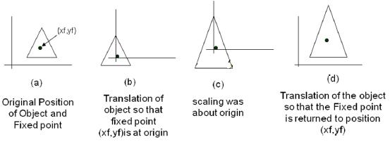
Concatenating the matrices for these three operations
produces the required scaling matix
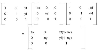
Can also be expressed as T(xf, yf).S(sx, sy).T(-xf, -yf) = S(xf, yf, sx,
sy)
Note: Transformations can be combined by matrix multiplication
Note: Transformations can be combined by matrix multiplication

Implementation of composite transformations
#include <math.h>
#include <graphics.h>
typedef float Matrix3x3 [3][3];
Matrix3x3 thematrix;
void matrix3x3SetIdentity (Matrix3x3 m)
{
int i,j;
for (i=0; i<3; i++)
for (j=0: j<3; j++ )
m[il[j] = (i == j);
}
/ * Multiplies matrix a times b, putting result in b */
void matrix3x3PreMultiply (Matrix3x3 a. Matrix3x3 b)
{
int r,c:
Matrix3x3 tmp:
for (r = 0; r < 3: r++)
for (c = 0; c < 3; c++)
tmp[r][c] =a[r][0]*b[0][c]+ a[r][1]*b[l][c] + a[r][2]*b[2][c]:
for (r = 0: r < 3: r++)
for Ic = 0; c < 3: c++)
b[r][c]=- tmp[r][c]:
}
void translate2 (int tx, int ty)
{
Matrix3x3 m:
rnatrix3x3SetIdentity (m) :
m[0][2] = tx;
m[1][2] = ty:
matrix3x3PreMultiply (m, theMatrix);
}
vold scale2 (float sx. float sy, wcPt2 refpt)
(
Matrix3x3 m.
matrix3x3SetIdentity (m);
m[0] [0] = sx;
m[0][2] = (1 - sx)* refpt.x;
m[l][l] = sy;
m[10][2] = (1 - sy)* refpt.y;
matrix3x3PreMultiply (m, theMatrix);
}
void rotate2 (float a, wcPt2 refPt)
{
Matrix3x3 m;
matrix3x3SetIdentity (m):
a = pToRadians (a);
m[0][0]= cosf (a);
m[0][1] = -sinf (a) ;
m[0] [2] = refPt.x * (1 - cosf (a)) + refPt.y sinf (a);
m[1] [0] = sinf (a);
m[l][l] = cosf (a];
m[l] [2] = refPt.y * (1 - cosf (a) - refPt.x * sinf ( a ) ;
matrix3x3PreMultiply (m, theMatrix);
}
void transformPoints2 (int npts, wcPt2 *pts)
{
int k:
float tmp ;
for (k = 0; k< npts: k++)
{
tmp = theMatrix[0][0]* pts[k] .x * theMatrix[0][1] * pts[k].y+ theMatrix[0][2];
pts[k].y = theMatrix[1][0]* pts[k] .x * theMatrix[1][1] * pts[k].y+ theMatrix[1][2];
pts[k].x =tmp;
}
}
void main (int argc, char **argv)
{
wcPt2 pts[3]= { 50.0, 50.0, 150.0, 50.0, 100.0, 150.0};
wcPt2 refPt ={100.0. 100.0};
long windowID = openGraphics (*argv,200, 350);
setbackground (WHITE) ;
setcolor (BLUE);
pFillArea(3, pts):
matrix3x3SetIdentity(theMatrix);
scale2 (0.5, 0.5, refPt):
rotate2 (90.0, refPt);
translate2 (0, 150);
transformpoints2 ( 3 , pts)
pFillArea(3.pts);
sleep (10);
closeGraphics (windowID);
}
Other Transformations
1. Reflection
2. Shear
Reflection
A reflection is a transformation that produces a mirror image of an object. The mirror image for a two-dimensional reflection is generated relative to an axis of reflection by We can choose an axis of reflection in the xy plane or perpendicular to the xy plane or coordinate origin
Reflection of an object about the x axis

Reflection the x axis is accomplished with the
transformation matrix

Reflection the y axis is accomplished with the
transformation matrix

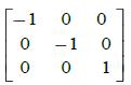
Reflection of an object about the coordinate origin

Reflection about origin is accomplished with the
transformation matrix
Reflection axis as the diagonal line y = x

To obtain transformation matrix for reflection about
diagonal y=x the transformation sequence is
1. Clock wise rotation by 450
2. Reflection about x axis
3. Counter clock wise by 450
Reflection about the diagonal line y = x is accomplished with the transformation matrix
1. Clock wise rotation by 450
2. Reflection about x axis
3. Counter clock wise by 450
Reflection about the diagonal line y = x is accomplished with the transformation matrix

Reflection axis as the diagonal line y = -x

To obtain transformation matrix for reflection about
diagonal y = -x the transformation sequence is
1. Clock wise rotation by 450
2. Reflection about y axis
3. counter clock wise by 450
Reflection about the diagonal line y = -x is accomplished with the transformation matrix
1. Clock wise rotation by 450
2. Reflection about y axis
3. counter clock wise by 450
Reflection about the diagonal line y = -x is accomplished with the transformation matrix

Shear
A Transformation that slants the shape of an object is called the shear transformation. Two common shearing transformations are used. One shifts x coordinate values and other shift y coordinate values. However in both the cases only one coordinate (x or y) changes its coordinates and other preserves its values.
X - Shear
The x shear preserves the y coordinates, but changes the x values which cause vertical lines to tilt right or left as shown in figure

The Transformations matrix for x-shear is

which transforms the coordinates as
x’ = x+x shx .y
y’ = y
Y - Shear
The y shear preserves the x coordinates, but changes the y values which cause horizontal lines which slope up or down
The Transformations matrix for y-shear is
x’ = x+x shx .y
y’ = y
Y - Shear
The y shear preserves the x coordinates, but changes the y values which cause horizontal lines which slope up or down
The Transformations matrix for y-shear is
which transforms the coordinates as
x’ = x
y’ = y + y shx .x
XY - Shear
The transformation matrix for xy-shear
x’ = x
y’ = y + y shx .x
XY - Shear
The transformation matrix for xy-shear

which transforms the coordinates as
x’ = x + x shx .y
y’ = y + y shx .x
Shearing Relative to other reference line
We can apply x shear and y shear transformations relative to other reference lines. In x shear transformations we can use y reference line and in y shear we can use x reference line.
X - shear with y reference line
We can generate x-direction shears relative to other reference lines with the transformation matrix


which transforms the coordinates as
x’ = x+x shx (yref y)
y’ = y
Example
Shx = ½ and yref = -1
x’ = x+x shx (yref y)
y’ = y
Example
Shx = ½ and yref = -1
Y - shear with x reference line
We can generate y-direction shears relative to other reference lines with the transformation matrix
We can generate y-direction shears relative to other reference lines with the transformation matrix
which transforms the coordinates as
x’ = x
y’ = shy (x - xref) + y
Example
Shy = ½ and xref = -1
x’ = x
y’ = shy (x - xref) + y
Example
Shy = ½ and xref = -1

Output primitives are the basic building blocks used in graphics rendering emailtooltester to represent geometric shapes like points, lines, and polygons. These are processed by the GPU to create visual elements on a screen.
ReplyDeleteOutput primitives are essential in graphics rendering, forming the foundation of complex visuals. For AI enthusiasts, the yolov8 architecture diagram can provide a clear understanding of how object detection models are structured and optimized.
ReplyDelete